![]()
![]()
![]()
![]()
Photometric Simulation
Note
This exact run can be started in the test of SEDobs. if you hit the command sedobs –test and select the photometric simulation sedobs will run exactly this configuration. An example of such can be downloaded here: link
Configuration
We describe here the process the SEDobs uses when doing a purely photometric simulation. The configuration we use is the one given below:
[General]
Project_name= SEDobs_Test_run_photometry
Author = R. THOMAS - 6/12/18
Project_Directory= ~/.sedobs/test_run_photo
full_array =
z_distribution = dist_z.txt
Nobj = 2500
sizegal = 1

[Data_Type]
Photometry = Yes
Spectro = No

[Spectro]
NSpec =
Norm_band =
Noise_reg =
Norm_distribution =
types =
flux_unit =
wave_unit =

[Photo]
Norm_band = (r-megacam,low,98)
Norm_distribution = dist_mag.txt
Nband = 10
Band_list = (u-megacam,0.0,0.31,0.38,low,98);(g-megacam,0.0,0.15,0.20,low,98);(r-megacam,0.0,0.19,0.09,low,98);(i-megacam, 0.0, 0.23, 0.12,low,98);(z-megacam,0.0, 0.38, 0.19,low,98);(J-wircam, 0.0, 0.68, 0.45,low,99);(H-wircam,0.0,0.71,0.37,low,99);(K-wircam,0.0,0.55,0.41,low,99);(IRAC1,0.0,0.08,0.04,none,100);(IRAC2,0.0,0.09,0.06,none,100)
flux_unit =
wave_unit =
savesky = No

[Cosmo]
Ho=70
Omega_m = 0.27
Omega_L = 0.73
Use_Cosmo = Yes

[Templates]
BaseSSP = LIB_BC03_Delayed_LR_Salp_SPARTAN.hdf5
DustModel = calzetti.dat
AvsList = 0.0;0.4050;0.8100;1.2149;1.6200;2.0250
RvsList = 4.05
IGMUse = SPARTAN_Meiksin_Free_7curves.hdf5
IGMtype = free
EMline= yes
EBVnList =
Lyafrac = 0.5
Age = 0.5e+08;0.75e+08;0.1e+09;0.2e+09;0.3e+09;0.4e+09;0.5e+09;0.6e+09;0.7e+09;0.8e+09;0.9e+09;1.0e+09;1.0e+09;1.1e+09;1.2e+09;1.3e+09;1.4e+09;1.5e+09
TAU = 0.10;0.2;0.3;0.4;0.5;0.6;0.7;0.8;0.9;1.0
MET = 0.4;1.0;2.5
We choose to use individual files (and not the full_array option).
Checking configuration
We starting sedobs with this file (sedobs -p simu.conf) sedobs start by checking your configuration. You can see the output of the terminal for the full checking of your configuration:
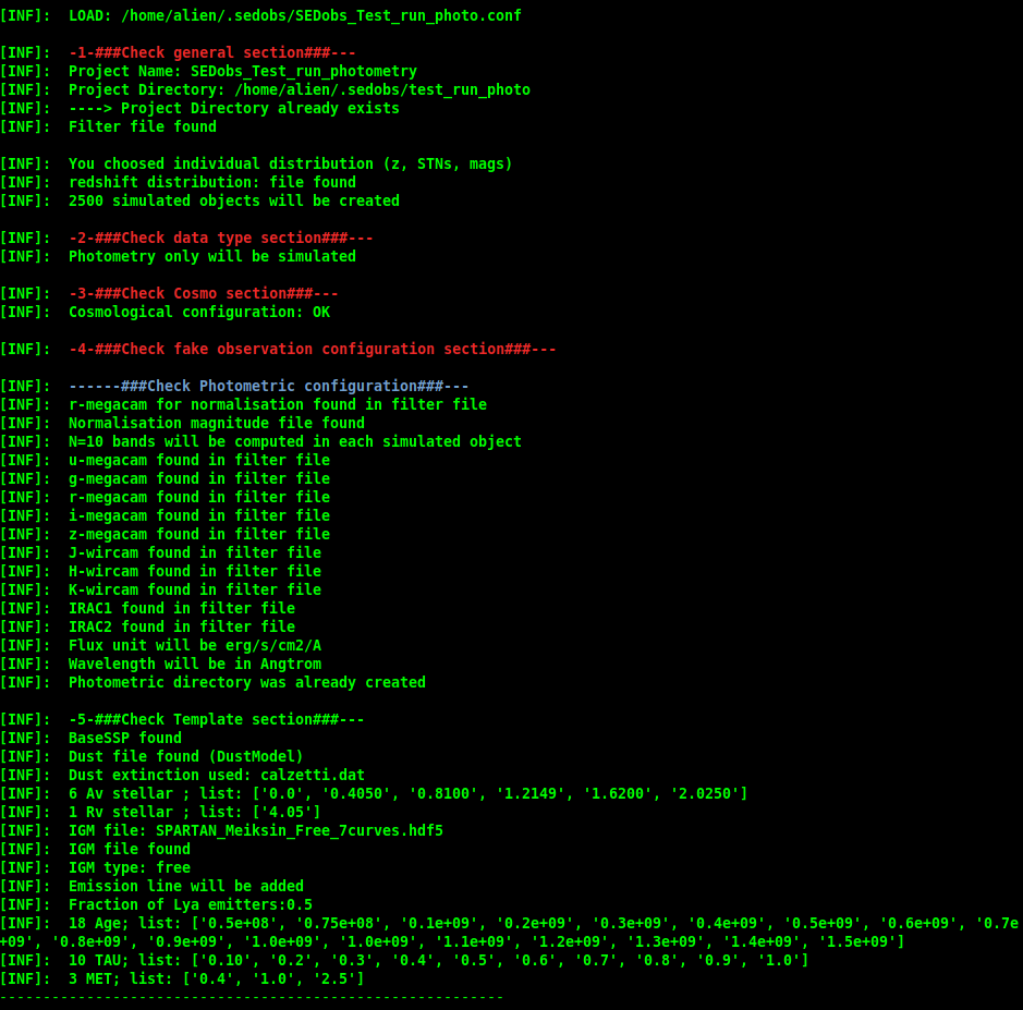
1-General section checking: First it tells you what file you loaded. Then it checks the general section of the configuration file. It makes sure that your directory exist and that the filter file is found. Since we do not give a full array, it assumes we give individual distribution (in the photometric case only the redshift distribution, and normalisation magnitude distribution). It checks that the redshift distribution is found and that the number of objects is given. In the project directory you will have this files:
Project Directory
    |_dist_z.txt
    |_dist_mag.txt
2-Check data type: Then SEDobs check what type of data you want to simulate.
3-Check Cosmology module: The cosmology configuration is verified
4-Check the photometric configuration: SEDobs then start to check the photometric configuration. It check the normalisation band and that the matgnitude distribution file is given (here dist_mag.txt). Then it looks at all the band that will be simulated.
5-Check template configuration: Then SEDobs look at your template setting. It checks that all the input files are found (IGM, dust extinction, templates).
Preparation
- After this checks, SEDobs is going to prepare the extra files:
The final redshift and normalisation magnitude distributions. From the two files given, two new distributions will be created (see above), matching the shape of the original ones with the number of object you want to create. These two distributions will joined in one file called ‘final_array_z_StN_mag.txt’ and placed in your project directory. This file can be re-used for another run using the final array option.
From the Ages, Tau and metallicities that you give in your configuration SEDobs recompute a library of templates and save it in SEDobs_Test_run_photometry.hdf5 (this name depends on the name of your project).
SEDobs starts to create the output files (with header). In this case it will be the parameter file, and the photometric file. It also creates the photo_indiv and original_template sub-directories.
Warning
if you change some of the template parameters (Age, Tau, met) you must delete the *.hdf5 file that was created previously because SEDobs try to look for an already computed library of template before creating one.
It is the same for the final_array_z_StN_mag.txt file. If you change your redshift distribution of your normalisation band distribution you have to delete this file. SEDobs try to look for it to check if one is already here. If it finds it it will not recalculate it.
Simulation
After all these checking and preparations SEDobs starts to simulate. For each object, SEDobs passes by different steps that are displayed in the terminal, an example is given below:
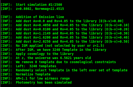
SEDobs start to take the library of templates that was created and add emission lines. If you asked to give a certain fraction of lyman alpha emitters it will take it into account. Then the dust extinction will be added and the IGM as well. SEDobs will also tell you how many templates there is after all extinction are applied. Next, it will apply the cosmology to the library. The templaes will be redshifted and if you decided to use the cosmology it will keep only the templates that are younger than the age of the universe at the redshift of the simulated galaxy.
The template used for the simulated galaxy will then be chosen randomly in the left over templates. It will be normalize to the normalisation magnitude value in the normalisation band you choosed and apply sky emission (if used) to the template. After that, all the band in your configuration are computed. In each band, the error is computed from the mean and sigma of the gaussian given for each band (see Configuration page).
Finally, everything is saved in different catalogs and single files(see Outputs for all the files that are created).
Note
This exact run can be started in the test of SEDobs. if you hit the command sedobs –test and select the photometric simulation sedobs will run exactly this configuration.