![]()
![]()
![]()
![]()
Atmospheric effect
In the spirit of making SEDOBS as complete as possible we implemented the sky emission. This has been made based on model computed for the Paranal Observatory. These modelisations are public and maintained by the European Southern Observatory (ESO). We use the v2.0.4 Cerro Paranal Advanced Sky Model (Available here). We detail below this effect and how it was implemented in SEDOBS in the following sections.
Sky Emission
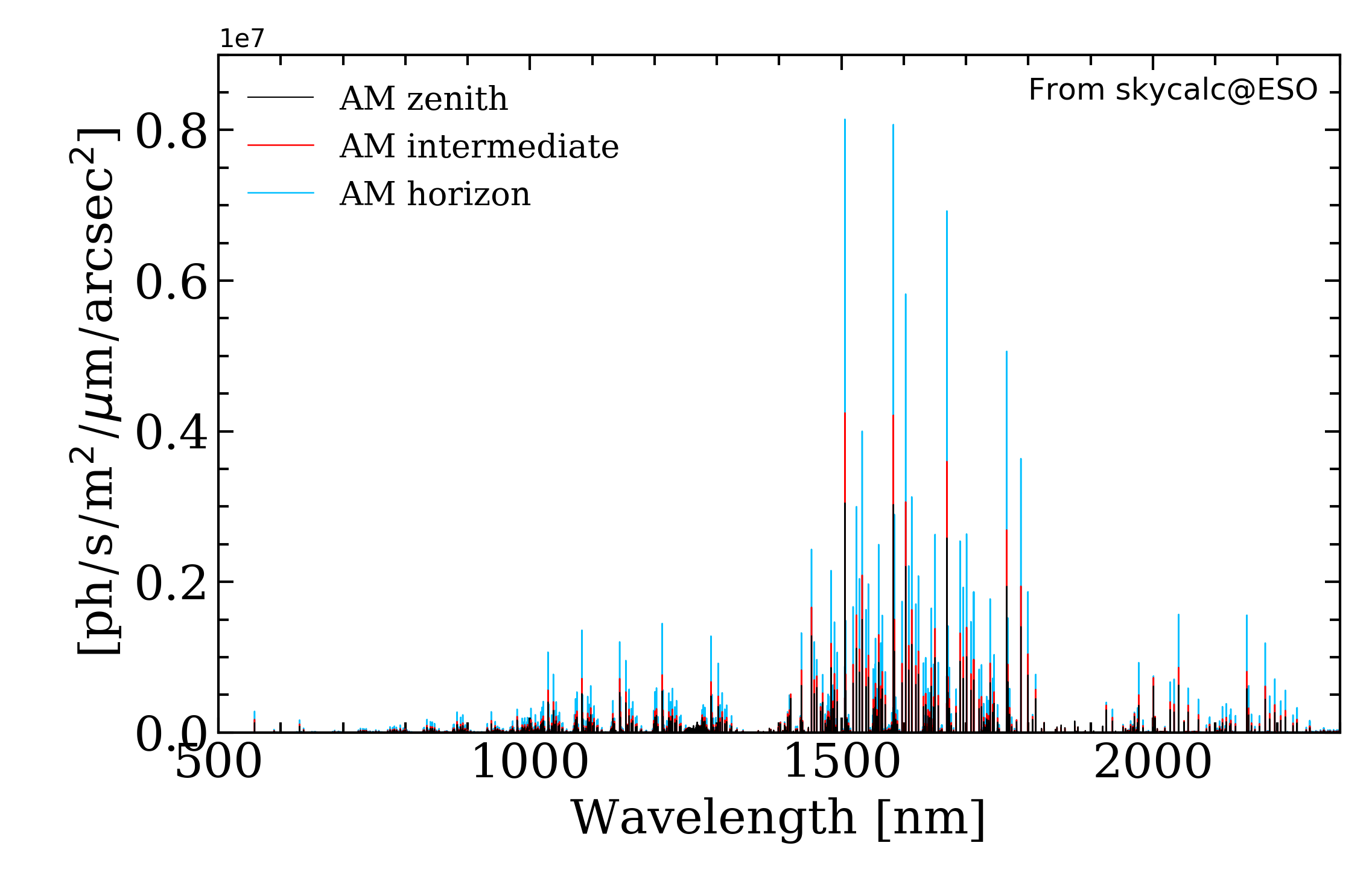
The earth atmosphere has a heavy impact on the flux reaching our ground-based observatories. Alongside the atmospheric absorption (not implemented here) you also have the possibility to use sky emission simulation to fake the sky subtraction during the reduction process. The sky model of Cerro Paranal produces the sky emission model. To create these models we asked for Scatterd Starlight, Zodiacal light, Molecular emission of Lower Atmospher, Emission lines of Upper atmosphere and airglow residual. We do not used the scattered moonlight as we assume dark time was used for real observation. As the data configuration can include both space and ground-based data the definition of observation place (ground or space) must be precised for each spectrum and/or band that is simulated (see Configuration for more details about how you have to tell SEDOBS in practice). SEDOBS as implemented three groups of AIRMASS ranges that can be used: low, intermediate and high. Using the low range will apply the attenuation considering AM between 1 and 1.15 (corresponding to altitudes between 90 degrees and 60.4 degrees). Using the intermediate range of airmass will assign randomly an AM between 1.15 and 1.4 (equivalent to altitudes of 60.4 degrees and 45.5 degrees). Finally, the high airmass range will be using airmasses above 1.4 up to 2.95 (altitude of 45.4 and 19.8 degrees, 19.5 degree being the limit of the model and below the pointing limit of the Unit telescopes of the VLT). The ESO modelisation provides the sky radiance in \([ph/s/m^2/\mu m/ arcsec^2]\) and can be seen in the figure below:
We convert this to \([erg/s/cm^2/Ang/arcsec^2]\) using:

where h, c and \(\lambda\) are the Planck’s constant, the speed of light and the wavelength. As we need to convert this to a flux density \([erg/s/cm^2/Ang]\) we need to consider an angular size in the sky for our galaxy. The default value is set to \(1''\). This value can be easily changed in the configuration file (see Configuration). When simulating photometry SEDOBS adds up the skyline spectrum to the synthetic spectrum before computing the magnitudes. In the case of spectroscopy, SEDOBS adapts the resolution of the skyline spectrum to the resolution of the simulated observation and then adds it up to the synthetic template as well. The noise estimation is then computed on the addition of the galaxy synthetic template and the skyline template.
Sky subtraction
Once the sky emission is added to the template you can simulate the sky subtraction. For each band/spectrum a number has to be given, between 0(%) and 100(%), which corresponds to the efficiency of the sky subtraction. The meaning of this percentage answers the question ‘how much sky can I get rid of during the data reduction’?. SEDOBS will then remove X quantity of the sky and will leave 1-X of sky residual in the spectrum. Of course, if you do not want to subtract the sky you can say that the sky subtraction is efficient at a level of 0%. If you do not want the sky at all then 100% of sky subtraction efficiency will do the trick.
Output
In case of Photometry the user has the choice of saving the sky spectrum that was used during the simulation. In that case, the sky spectrum is limited to the wavelength range encompassing the magnitude at the smallest wavelength and the one at the highest wavelength. In the case of spectroscopy, the choice is not given to the user and the sky spectrum is automatically saved for each spectrum it was used. It is saved at the same resolution of the simulated spectrum and in the same wavelength grid.